Performance Prediction and MgCl Setpoint Adjustment of a Utility-Scale Struvite Precipitation Reactor
Project overview video
Define Problem:
Metro Water Recovery (MWR) in Denver, CO uses enhanced biological phosphorus removal (EBPR) to remove phosphorus from their main treatment stream. During subsequent anaerobic digestion (AD) of the EBPR sludge, a portion of the biomass-bound phosphorus is re-solubilized and released into the sidestream of the plant. This high concentration of phosphorus leads to inadvertent struvite precipitation that causes scaling in pipes and fixtures (Figure 1) resulting in operational shutdowns and increased maintenance costs. Additionally, after recycling of the sidestream into the main stream, the phosphorus loading of the plant actually increases over time.

Figure 1. Images of struvite scaling on pipes at MWR’s facility
To address these issues and help meet effluent discharge limits, MWR uses a controlled struvite precipitation reactor. These reactors transform soluble orthophosphate (OP) in the anaerobic digester effluent into struvite (NH4MgPO4 6H2O) precipitate, enabling the removal and recovery of phosphorus as well as protecting critical infrastructure from scaling. In 2020, MWR installed a commercial struvite precipitation reactor to treat their AD effluent prior to sludge dewatering and sidestream recycling. The key control variables for the system are the MgCl dosage and the rate of aeration for pH control (Figure 2).

Figure 2. Diagram of the MagPrex® system installed at MWR. The key control variables are boxed in red.
Currently, MWR is adjusting their MgCl dosage based on a 1.3:1 Mg-P ratio with weekly orthophosphate (OP) measurements from the AD digestate. Due to the extended time it takes to obtain the OP laboratory measurements, MWR is unable to get an accurate, real-time understanding of the reactor’s performance and adjust set points accordingly. Furthermore, laboratory experiments can be expensive and time consuming. Costs, maintenance requirements, and inaccuracies in measuring OP concentrations in the complex digestate matrix have prevented adoption of commercially available sensors and online analyzers that could help with optimizing control processes. An investigation into leveraging a variety of statistical and machine learning (ML) methods is therefore undertaken to provide daily predictions for the influent OP, effluent OP, and OP removed from the reactor and to recommend MgCl setpoints (MgCl SP) that would lead to MWR’s ideal reactor effluent OP concentration of 30 mg P/L.
Go/No-Go Decision: If your problem can be accurately modeled with a mechanistic model, improved by operator staff training, or if existing data collection infrastructure is not in place then data-driven modeling may not be the right solution.
Get Data:
Over 15 months, MWR collected a dataset spanning 95 variables and 439 days. 65 variables were laboratory measurements (e.g., digester effluent magnesium and OP concentrations) with observations generally occurring 1-3 times a week. 30 variables were online measurements (e.g., pH and MgCl feed) with a time weighted, average observation occurring every day. All of the laboratory and online measurements were pulled from MWR’s internal data collection system into separate MS Excel files. These Excel files were then imported into Python, merged together, and matched up by timestamp.
Prior to moving forward with prepping the data and building the models, it was important to start with some exploratory data analysis (EDA) to better understand the dataset that was collected. EDA typically involves plotting histograms, scatterplots (Figure 3) , and boxplots of individual variables in a dataset to help quickly identify diagnostic information and plan out next steps. We plotted key variables of interest to make sure we had enough variation in our data to justify modeling them. Of these key variables, we found that the aeration blower used to control pH was turned off for the majority of the data collection timeline. While initially we were interested in modeling a blower set point model, due to this lack of data, we instead focused on developing influent OP, effluent OP, and OP removal models.

Figure 3. Initial scatter plots of key operational data.
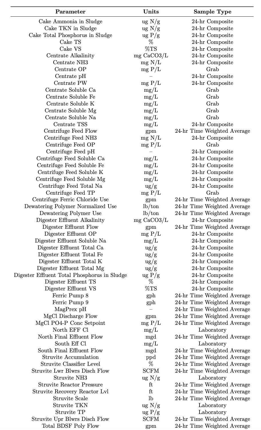
Figure 4. List of the types of variables that were monitored
Go/No-Go Decision: ML may not be a viable solution to your problem if your dataset contains a majority of missing or constant data. If your dataset contains data with little variance then your ML models may not perform any better than taking the statistical mean of the data.
Prepare Data:
An important step in any data-driven modeling process, is to clean and process the raw dataset. Laboratory measurements are typically taken at various timestamps throughout the day, so we resampled the dataset to combine all observations within the same day into a single row of daily observations. We then removed any row in the dataset that did not include values for digester effluent OP (influent OP into the reactor), centrifuge feed OP (effluent OP out of the reactor), and MgCl discharge (indicator that the system was online) to ensure a baseline amount of knowledge on the system’s performance was included. Additional variables were removed that had the vast majority of their observations missing or constant.
After this initial data cleaning, we focused attention towards outlier removal and data imputation. Through EDA and consultation with MWR’s process engineers, we began by manually identifying known outliers in the dataset. We then used kernel density estimation (KDE) with a gaussian kernel to fit probability density curves to each individual variable’s data (Figure 5). We iteratively adjusted the bandwidth and significance level (cutoff for what is considered an outlier or not) of the KDE until the known outlier points were identified. Resultantly, an observation from each feature was identified as an outlier when it had a log probability less than the 10th percentile. All manually and statistically identified outlier observations were then set equal to N/A.
Due to the outlier removal process and the infrequency of laboratory measurements, several rows of timestamps included missing or N/A observations. Imputation was thus performed to fill in unavailable data. The last-observation-carried-forward technique, which assumes data on days with missing observations is equal to the value of the last measured observation, was used first. For any remaining missing observations, data was backfilled with the first available measurement. Once imputation was finished, OP removal values which equal the difference between the influent OP and the effluent OP concentrations were added to the dataset as an additional variable and any remaining outliers were removed using the IQR method. Our final dataset consisted of 87 variables and 152 observations.

Figure 5. Visual summary of the data prep steps
Go/No-Go Decision: ML modeling performs best with a large amount of observations. If your dataset has more variables than observations or a small set of observations that do not capture the variability of your process then you may not want to proceed.
Model Selection and Training:
Six modeling methods were evaluated on predicting three different objective variables: influent OP, effluent OP, and OP removal. To prevent data leakage by giving the models extra information that could cause over-optimistic predictions, the objective variables and other OP-related data were dropped from the independent variable set. For this write up, the influent and effluent OP predictions are used as examples. To see results from OP removal predictions, visit the main project website.
#define X and y variables

y_inf = df['Dig Eff OP']
y_eff = df['Cent Feed OP']

#drop variables that are closely related to the objective variables
X = df.drop(['OP Removed', 'Dig Eff OP', 'Cent Feed OP', 'Centrate OP',
'MgCl PO4 P Conc SP', 'Centrate PW'], axis = 1)
Before moving on to more computationally complex ML modeling methods, it is often good practice to evaluate whether simpler and more easily interpretable statistical models can be effective at meeting your objective. Four different types of statistical regression modeling methods including linear regression (LR), partial least squares (PLS), ridge, and lasso regression were therefore evaluated.
#define function to create a linear regression model
def lin_reg():
   lr_model = LinearRegression()
   return lr_model

#define function to create a partial least squares regression model
def pls_reg():
   pls_model = PLSRegression(n_components = 2)
   return pls_model

#define function to create ridge model
def ridge_CV(X_train, y_train, cv):
   #create a large range of alpha values to test for CV
   alphas = 10**np.linspace(10,-2,100)*0.5
   #find a tuned alpha value using cross validation
   ridgecv = RidgeCV(alphas, cv=cv)
   ridgecv.fit(X_train, y_train)
   #define the tuned model
   ridgecv_model = Ridge(alpha=ridgecv.alpha_)
   return ridgecv_model #return the pre-fitted, tuned model

#define function to create lasso model
def lasso_CV(X_train, y_train, cv):
   #find a tuned alpha value using cross validation
   lassocv = LassoCV(cv=cv, tol = 0.009)
   lassocv.fit(X_train, y_train)
   #define the tuned model
   lassocv_model = Lasso(alpha=lassocv.alpha_)
   return lassocv_model #return the pre-fitted, tuned model
To see if ML is a more effective modeling tool for this case, eXtreme Gradient Boosting (XGBoost) was evaluated as well. A baseline model utilizing the mean values of the OP removal and the MgCl SP data for predictions was also developed as a point of comparison for all other models.
For the ridge, lasso, and XGBoost models there are a variety of model hyperparameters that can be tuned to improve prediction accuracies. For our ridge and lasso models, cross validation was used to identify ideal alpha values from the training data. For the XGBoost model, which has several more hyperparameters, a bayesian tuner was used instead.
#Define XGBoost Regression model
#define the model architecture
def xgb_feat(hp):

  #XG Boost hyperparameter boundaries for exploration by the tuner.
  #The parameters to tune are limited for simplification purposes
  min_max_depth = 3
  max_max_depth = 8
  min_eta = 0.001
  max_eta = 0.5
  min_n_estimators = 100
  max_n_estimators = 300


  xgb_feat = XGBRegressor(
    max_depth=hp.Int('max_depth', min_value=min_max_depth, max_value=max_max_depth, step=1),
    eta=hp.Float('eta', min_value=min_eta, max_value=0.5, sampling='log'),
    n_estimators=hp.Int('n_estimators', min_value=min_n_estimators,
    max_value=max_n_estimators, step = 10),
    colsample_bytree=0.8,
    subsample=0.5,
    min_child_weight=1,
    gamma=0.005,
    reg_lambda=1,
    reg_alpha=0,
    objective="reg:squarederror"
    )

  #To expand your hyperparameter boundaries use the following code
  #Note this will significantly increase your compiling time in later steps
  # xgb_feat = XGBRegressor(
  #   max_depth=hp.Int('max_depth', min_value=3, max_value=10, step=1),
  #   eta=hp.Float('eta', min_value=0.0001, max_value=0.5, sampling='log'),
  #   learning_rate=hp.Float('eta', min_value=0.0001, max_value=0.5, sampling='log'),
  #   n_estimators=hp.Int('n_estimators', min_value=10, max_value=500, step = 10),
  #   colsample_bytree=hp.Float('colsample_bytree', 0.1, 1, sampling='linear'),
  #   subsample=hp.Float('subsample', 0.1, 1, sampling='linear'),
  #   min_child_weight=hp.Int('min_child_weight', 1, 6, sampling='linear'),
  #   gamma= hp.Float('gamma', 0.001, 0.5, sampling='log'),
  #   reg_lambda=hp.Float('reg_lambda', 1e-3, 1, sampling='log'),
  #   reg_alpha=hp.Float('reg_alpha', 1e-3, 1, sampling='log'),
  #   objective="reg:squarederror"
  #   )

  return xgb_feat

#Build the XGBoost Model
def xgb_mod(X_train, y_train):
  #build the hyperparameter tuner
  xgb_feat_tuner = kt.tuners.SklearnTuner(
      oracle=kt.oracles.BayesianOptimizationOracle(
          objective=kt.Objective('score', 'min'),
          max_trials=5), #note you can increase max_trials to identify more ideal hyperparameters (this will increase your compile time)
      hypermodel=xgb_feat,
      scoring=make_scorer(mean_squared_error),
      project_name='xgb_feat_model_tuner_files',
      overwrite=True
  )

  #search across the sample space for the best hyperparameters
  xgb_feat_tuner.search(X_train, y_train.values)

  xgb_model = xgb_feat_tuner.get_best_models(num_models=1)[0]

  return xgb_model  #return the pre-fitted, tuned model
To evaluate each model on its ability to predict a variety of unseen data, a repeated k-fold cross validation with five folds and one repeat was used to split up the processed dataset (Figure 6). The root mean squared error (RMSE) between the actual measured Y variable data and the predicted Y variable data from each of the cross validation splits was calculated and averaged to provide a score for all models. The standard error (SEM) of the average RMSE values was also calculated.

Dimension Reduction:
Given the large number of variables in our dataset compared to the number of observations, a variety of dimension reduction methods were investigated to reduce model complexity and filter noise. A comparison between three different dimension reduction techniques, Spearman’s correlation (ρ), Principal Component Analysis (PCA), and Maximum Relevance-Minimum Redundancy (mRMR), was undertaken. Additional techniques used in the full project can be found in the write-up on the main project website.
ρ is a nonparametric variation measuring the strength and direction of monotonic relationships. The correlations of all variables to the Y variables were found using ρ and the lowest correlated variables were removed.
#Define a function to identify highly correlated features using
#spearman's rho (pairwise correlation) for removal
def identify_sp_correlated(X, y, threshold):
  # Calculate Spearman's rho for each feature with the target variable
  correlations = X.apply(lambda col: spearmanr(col, y).correlation)

  # Get the # of features with the highest absolute Spearman correlation
  top_features = correlations.abs().nlargest(threshold+1)
  top_features = top_features.iloc[1:]

  return top_features #return the top correlated features to keep
PCA involves creating linear combinations of existing variables to sequentially capture the most variation in the data. Across these linear combinations (i.e, principal components), those variables with the lowest contributions to the variations in the data were removed.
#Define a function to identify variables for removal using PCA
def identify_pca(df, pred_var, threshold):
  Xtrain = df
  Xtrain.loc[:,'y'] =  pd.Series(pred_var, index=Xtrain.index)

  # Apply standard scaler
  scaler = StandardScaler()
  Xtrain= scaler.fit_transform(Xtrain)

  # Fit PCA model
  cov_matrix = np.cov(Xtrain, rowvar=False)
  egnvalues, egnvectors = np.linalg.eigh(cov_matrix)
  total_egnvalues = sum(egnvalues)
  var_exp = [(i/total_egnvalues) for i in sorted(egnvalues, reverse=True)]
  var_exp = pd.DataFrame (var_exp)
  egnpairs = [(np.abs(egnvalues[i]), egnvectors[:, i]) for i in range(len(egnvalues))]
  egnpairs.sort(key=lambda k: k[0], reverse=True)

  # All PCs
  projectionMatrix = np.hstack([(egnpairs[i][1][:, np.newaxis]) for i in range(len(egnvalues))])
  proj_mat = abs(pd.DataFrame(projectionMatrix, columns =['PC'+str(i) for i in
  range(1,len(egnvalues)+1)], index=df.columns))

  # Find PCs where Predictive Variable is significant.
  which = lambda lst:list(np.where(lst)[0])
  col_ls = []
  col = list(proj_mat)
  for i in col:
      df = proj_mat[i].sort_values(ascending = False)
      df = df[df>0.05]
      if any('y' == df.index):
          new_df = pd.DataFrame(df.index)
          new_df['PC_Variance'] = [var_exp.iloc[which(proj_mat.columns==i),0].values[0] for x in range(len(new_df.index))]
          col_ls.append(new_df)

  # Aggregate weights of variables across PCs.
  col_df = pd.concat(col_ls)
  col_df = col_df.groupby([0])['PC_Variance'].sum()

  col_df = col_df.sort_values(ascending=False)
  col_df = col_df.drop(['y'])
  return col_df.head(threshold).index.values #return the column names to keep
For mRMR, a ranking based on F-scores and correlation coefficients was created and the highest scoring variables were kept.
#%%Define a function to select features using MRMR method
#edited from https://towardsdatascience.com/mrmr-explained-exactly-
#how-you-wished-someone-explained-to-you-9cf4ed27458b
def identify_mrmr(X, y, threshold):
    # compute F-statistics and initialize correlation matrix
    F = pd.Series(f_regression(X, y)[0], index = X.columns)
    corr = pd.DataFrame(.00001, index = X.columns, columns = X.columns)

    # initialize list of selected features and list of excluded features
    selected = []
    not_selected = X.columns.to_list()

    # repeat threshold times
    for i in range(threshold):

        # compute (absolute) correlations between the last selected feature
        #and all the (currently) excluded features
        if i > 0:
            last_selected = selected[-1]
            corr.loc[not_selected, last_selected] =
            X[not_selected].corrwith(X[last_selected]).abs().clip(.00001)

        # compute FCQ score for all the (currently) excluded features
        score =
        F.loc[not_selected] / corr.loc[not_selected, selected].mean(axis = 1).fillna(.00001)

        # find best feature, add it to selected and remove it from not_selected
        best = score.index[score.argmax()]
        selected.append(best)
        not_selected.remove(best)

    return selected #return the column names to keep
To identify the best performing dimension reduction technique and ideal number of variables to keep, the six modeling approaches were trained and tested on different numbers of variables. Training occurred on the first five variables selected and then was repeated for five additional variables until 30 were selected, this process was repeated for each of our dimension reduction techniques.
#create a repeated k fold with 5 splits and 1 repeat.
#For a more robust evaluation, consider increasing the number of repeats.
rkfcv = RepeatedKFold(n_splits=5, n_repeats=1, random_state=50)
rkfcv.get_n_splits(X, y_inf)

#array with list of models being run
models = ['mean', 'lr', 'pls', 'ridgeCV', 'lassoCV', 'xgb']

#creating dataframes to add rmse and prediction results into
inf_rmse_results_df = pd.DataFrame()
eff_rmse_results_df = pd.DataFrame()
inf_train_predict_results_df = pd.DataFrame()
inf_test_predict_results_df = pd.DataFrame()
eff_test_predict_results_df = pd.DataFrame()
eff_train_predict_results_df = pd.DataFrame()

train_predict_results_arr = [inf_train_predict_results_df, eff_train_predict_results_df]
test_predict_results_arr = [inf_test_predict_results_df, eff_test_predict_results_df]
rmse_results_arr = [inf_rmse_results_df, eff_rmse_results_df]
y_arr = [y_inf, y_eff]

# loops through all of the training and testing data as defined by the repeated k fold
for i, (train_index, test_index) in enumerate(rkfcv.split(X)):
    j=0
    for y in y_arr: #loops through and models all of the objective variables
      rmse_results = pd.DataFrame()
      train_predict_results = pd.DataFrame()
      test_predict_results = pd.DataFrame()
      X_train = X.iloc[train_index]
      y_train = y.iloc[train_index]
      X_test = X.iloc[test_index]
      y_test = y.iloc[test_index]

      #scale data
      sc = StandardScaler()
      X_train_scaled = sc.fit_transform(X_train)
      X_train_scaled = pd.DataFrame(data=X_train_scaled, columns=X_train.columns)
      X_test_scaled = sc.fit_transform(X_test)
      X_test_scaled = pd.DataFrame(data=X_test_scaled, columns=X_test.columns)

      for model_type in models: #loops through all four modeling methods
        train_predict_arr = []
        test_predict_arr = []
        test_rmse = []
        features_kept = []
        #loop through the first 30 variables
        for num in range(5, 35, 5): #to go through the entire variable list replace 35 with len(X_train.columns.values)+5
          #Create feature selection dataset with varying number of features
          selected_cols = identify_mrmr(X_train, y_train, num)

          X_train_feat = X_train_scaled[selected_cols] #using the selected features redefine the X_training and testing data
          X_test_feat = X_test_scaled[selected_cols]
          if model_type == 'mean':
              train_predict = pd.DataFrame([np.mean(y_train)]*len(y_train), columns=[''])
              test_predict = pd.DataFrame([np.mean(y_test)]*len(y_test), columns=[''])
          else:
            if model_type == 'lr':
                model = lin_reg()
            elif model_type == 'pls':
                model = pls_reg()
            elif model_type == 'ridgeCV':
                model = ridge_CV(X_train_feat, y_train, rkfcv)
            elif model_type == 'lassoCV':
                model = lasso_CV(X_train_feat, y_train, rkfcv)
            elif model_type == 'xgb':
                model = xgb_mod(X_train_feat, y_train)

            model.fit(X_train_feat, y_train) # Fit model and get predictions on test data

            train_predict = model.predict(X_train_feat)
            test_predict = model.predict(X_test_feat)

          train_predict_results[f"{model_type}_{num}_train"] = train_predict # store the prediction results in a dataframe
          test_predict_results[f"{model_type}_{num}_test"] = test_predict

          test_rmse.append(mean_squared_error(y_test, test_predict, squared=False)) # store the rmse results
          features_kept.append(num)

        train_predict_results[f"y_train"] = y_train.values
        test_predict_results[f"y_test"] = y_test.values

        rmse_results["features_kept"] = features_kept
        rmse_results[f"{model_type}_testing_rmse"] = test_rmse

      train_predict_results_arr[j] = pd.concat([train_predict_results_arr[j], train_predict_results], ignore_index=True, axis=0)
      test_predict_results_arr[j] = pd.concat([test_predict_results_arr[j], test_predict_results], ignore_index=True, axis=0)

      rmse_results_arr[j] = pd.concat([rmse_results_arr[j], rmse_results], ignore_index=True, axis=0)
      j+=1

#save training, testing, and rmse results
train_predict_results_arr[0].to_pickle('/content/drive/MyDrive/Workbook/inf_mrmr_train_results.pkl')
train_predict_results_arr[1].to_pickle('/content/drive/MyDrive/Workbook/eff_mrmr_train_results.pkl')

test_predict_results_arr[0].to_pickle('/content/drive/MyDrive/Workbook/inf_mrmr_test_results.pkl')
test_predict_results_arr[1].to_pickle('/content/drive/MyDrive/Workbook/eff_mrmr_test_results.pkl')

rmse_results_arr[0].to_pickle('/content/drive/MyDrive/Workbook/inf_mrmr_rmse_results.pkl')
rmse_results_arr[1].to_pickle('/content/drive/MyDrive/Workbook/eff_mrmr_rmse_results.pkl')
Figure 6. Visual representation of a repeated k-fold cross validation process. Adapted from Sontakke et al. 2019. Classification of Cardiotocography Signals Using Machine Learning: Proceedings of the 2018 Intelligent Systems Conference.
Analyze Results:
The results from each dimension reduction technique and model evaluation were averaged and plotted for comparison (Figure 7).
models = ['mean', 'lr', 'pls', 'ridgeCV', 'lassoCV', 'xgb']

inf_rmse_results_arr = [inf_sp_rmse_results_df, inf_pca_rmse_results_df,
                        inf_mrmr_rmse_results_df]
eff_rmse_results_arr = [eff_sp_rmse_results_df, eff_pca_rmse_results_df,
                        eff_mrmr_rmse_results_df]
feat_selec_arr = [inf_rmse_results_arr, eff_rmse_results_arr]

avg_results_arr = []

for results_arr in feat_selec_arr:
  for results_df in results_arr:
    avg_results_df = pd.DataFrame()
    for model_type in models:
      avg_test_rmse_results = []
      avg_test_se_results = []
      features_kept = []
      for num in results_df['features_kept'].unique():
        num_results = results_df[results_df['features_kept']==num]
        avg_test_rmse_results.append(np.mean(num_results[f"{model_type}_testing_rmse"]))
        avg_test_se_results.append(sem(num_results[f"{model_type}_testing_rmse"]))
        features_kept.append(num)

      avg_results_df["features_kept"] = features_kept
      avg_results_df[f"{model_type}_testing_rmse"] = avg_test_rmse_results
      avg_results_df[f"{model_type}_testing_se"] = avg_test_se_results

    avg_results_arr.append(avg_results_df)
colors = ['b', 'g', 'r', 'c', 'm', 'y']
fig, ([ax1, ax2, ax3], [ax4, ax5, ax6]) = plt.subplots(2, 3, figsize=(20, 10))
axes = [ax1, ax2, ax3, ax4, ax5, ax6]
j = 0
for ax in axes:
i = 0
ymin = 50
help_str = "testing"
average_rmse_results = avg_results_arr[j]
for model in models:
ax.errorbar(average_rmse_results['features_kept'], average_rmse_results[model+'_'+help_str+'_rmse'],
yerr=average_rmse_results[model+'_'+help_str+'_se'], color=colors[i])
ax.plot(average_rmse_results['features_kept'], average_rmse_results[model+'_'+help_str+'_rmse'], '-o', label=model+' '+help_str, color=colors[i])
i+=1
if average_rmse_results[model+'_'+help_str+'_rmse'].min() < ymin:
ymin = average_rmse_results[model+'_'+help_str+'_rmse'].min()
xpos = np.where(average_rmse_results[model+'_'+help_str+'_rmse'] == ymin)
xmin = average_rmse_results['features_kept'][xpos[0]]
min_model = model
percent_improvement = ((average_rmse_results['mean_testing_rmse'].min() - ymin)/average_rmse_results['mean_testing_rmse'].min())*100
ax.plot(xmin, ymin, '-o', color='black', zorder=10)
ax.annotate(f'Best performing model = {min_model}\nMin RMSE = {round(ymin, 1)}\nFeatures Kept = {xmin.values[0]}\nMean Improvement = {round(percent_improvement,1)}%', xy =(5, 45), fontsize=11)
ax.legend(loc='upper right')
ax.set_ylim(0,60)
ax.tick_params(axis='y', labelsize=15)
ax.tick_params(axis='x', labelsize=15)
if(j == 0 or j == 3):
feat_selec_type = "SP"
elif(j == 1 or j == 4):
feat_selec_type = "PCA"
elif(j == 2 or j == 5):
feat_selec_type = "mRMR"
ax.set_xlabel(xlabel=f'Features Kept ({feat_selec_type})', fontsize=15)
if(j < 3):
ax.set_ylabel(ylabel='RMSE of Influent OP (mg-P/L)', fontsize=15)
elif(j < 6):
ax.set_ylabel(ylabel='RMSE of Effluent OP (mg-P/L)', fontsize=15)
j+=1
Figure 7. Plotted RMSE results across model types and dimension reduction technique used. The first row shows results for the Influent OP predictions and the second row shows results for the Effluent OP predictions
For the influent OP predictions, selecting 20 variables with the mRMR method and using the linear regression model resulted in a minimum RMSE of 22.4 mg-P/L representing a 32.3% improvement over the mean model. For the effluent OP predictions, selecting 30 variables with PCA and using the XGBoost model resulted in a minimum RMSE of 12.2 mg-P/L representing a 53.6% improvement over the mean model.
These improvements over the mean help to justify the use of data driven modeling for predicting the objective variables and indicate MWR can reduce the number of monitored variables while maintaining similar or lower errors. Across the dimension reduction techniques and when considering all modeling types, there is little difference in RMSE values after the selection of 5 or more variables. This suggests a few key variables are influencing the majority of the predictive abilities of the models and that the type of dimension reduction technique used will be most influential when selecting a relatively small number of variables to keep.
In terms of model types, XGBoost resulted in the lowest RMSE values for every scenario except one indicating it as a preferred model for minimizing error during deployment. Interestingly though, the statistical models’ RMSE values for both the Influent and Effluent OP predictions were not far off and could be used going forward if the computational complexity of XGBoost is deemed not worth the lower prediction errors.
As can be seen in Figure 8, both the Influent and Effluent OP models fit the trend of the actual data relatively well but struggle to accurately predict values at the extremes of the data set. At the lower end of the concentration range, the models tend to overpredict and vice versa at the higher end of the range.

Figure 8. Plots of the predicted values versus the actual measured values. The left plot shows the Influent OP model results using mRMR dimension reduction and a linear regression model. The right plot shows the Effluent OP model results using PCA dimension reduction and an XGBoost model.
Go/No-Go Decision: If there is no meaningful improvement in model predictions over the mean, if the variables selected do not make physical sense, or if the models are severely overfit or do not capture data trends well, then you may need to reevaluate your data collection process or modeling objectives.
Deploy Models:
Deployment involved operationalizing the model code and integrating it with MWR’s internal data historian system. Python scripts were created to pull new data every day from the historian, integrate it with the historical raw data, and process it following the same procedures used during development and training. Code for predicting the three modeling objectives and MgCl SP recommendations were also created. MgCl SP recommendations were obtained using the predicted OP concentration data multiplied by MWR’s 1.3:1 Mg-P ratio. To sufficiently capture changes in data while conserving computing power, it was determined that model retraining on any new data would occur every two weeks. Prediction outputs were set up to publish results back to the historian and be shown to MWR engineers and operators. Laboratory OP tests continued to be run to help validate the deployed model predictions.
Go/No-Go Decision: If water quality changes not captured in the original dataset lead to worsening model results or if deployed code generally performs worse than expected, consider retraining the models, reevaluating your data collection process, or changing your modeling objectives.
Code overview video. Link to access code.