Biological Nutrient Removal: ABAC / AvN + PdNA

Project overview video

Code overview video. Link to access code.

Define Problem:

The facility where the data originated for this modelling exercise is the Hampton Roads Sanitation District (HRSD) Nansemond Treatment Plant (NTP). At the HRSD NTP, there is a biological process Digital Twin (DT) that regularly predicts the ammonia (NHx) concentrations at the end of the Aeration Tanks (ATs). The NHx concentrations are also measured with analyzers and so, an error can be determined between the modelled concentration and the measured concentration. In this exercise, we are attempting to forecast the mechanistic model error one Hydraulic Residence Time (HRT) into the future and leverage that forecast for improved Ammonia-Based Aeration Control (ABAC). This is considered a hybrid approach because it combines mechanistic and data-driven components into one.

This is also considered a multiple input single output (MISO) approach because we use the current error and rolling statistical information to forecast a single error into the future. The exercise below is partly to determine what MISO model is the ideal performer in terms of forecasting “extreme” values, or daily peaks and valleys in the mechanistic model error.

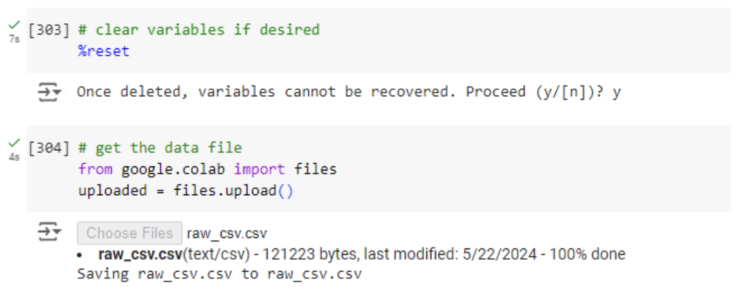
First, we break up our code into sections. The following sections are used here: SETUP, DATA PREP, MODELLING PREP, LINEAR REGRESSION, SIMPLE XG BOOST, TUNED XG BOOST, SIMPLE LSTM, TUNED LSTM, INITIAL RESULTS, and FAST FOURIER TRANSFORM. Before we even get to SETUP, we import the raw data file (raw_csv.csv) from a local folder. Any user repeating this exercise will need to save the raw_csv.csv file somewhere on their computer where they can easily access it.

Get Data:

Before we even get to SETUP, we import the raw data file (raw_csv.csv) from a local folder. Any user repeating this exercise will need to save the raw_csv.csv file somewhere on their computer where they can easily access it.

Under SETUP, we bring the data into a dataframe and call it X_raw. The timeframe being used for model training begins in October of 2023. During this time, 3 ATs were in service (at4, at6, and at7). This being the case, we can train on 2 of those tanks and then test on the 3rd. Temporally, we can also train on the first 80% of the dataset and test on the last 20%. This is a robust approach to ensuring that there is no data leakage from the training set to the test set. Before we move to the next step, we must decide what tanks will serve as the training and validation tanks and what tank will serve as the test tank.

# import required libraries/modules for SETUP
import pandas as pd
import numpy as np
import io
import matplotlib.pyplot as plt

# put the raw data into a dataframe
X_raw = pd.read_csv(io.BytesIO(uploaded['raw_csv.csv']))

# give X_raw a date/time index
X_raw['dt_index'] = pd.to_datetime(X_raw['dt_index'])
X_raw.set_index('dt_index', inplace=True)

all_tanks = ['at4', 'at6', 'at7']
train_val_tanks = ['at4', 'at7']
test_tank = ['at6']

Prepare Data:

With the tanks selected for their purpose, we will do a little bit of data cleaning and data preparation. First, we need to import the appropriate libraries. Those libraries/modules only include scipy.signal (savgol_filter), sklearn.model_selection (train_test_split), and sklearn.preprocessing (MinMaxScaler). With those libraries imported, we will begin by interpolating any missing values and smooth the data with a Savitzky-Golay filter to remove any noise. We also define the number of time steps that make up the average HRT because this is how we find the “future” errors that we are forecasting or the “y”s. The average HRT is 2 hours and 20 minutes and the time steps used here are 20 minutes, which is the amount of time it takes to measure the NHx with the analyzers at the ends of the aeration tanks. Therefore, hrt_time_steps = 7.

There are a couple items worth mentioning before moving on. One is that X are simply past values of y. This is evident by the .shift() piece of code. The other is that data quality was verified through visual inspection of the time series plots in MS Excel before beginning this coding exercise. The inspection focused on identifying high rates-of-change (changes in the noise pattern), magnitudes not possible, fixed-value faults, and abnormal signals that did not align with abnormalities in other signals simultaneously.

# import required libraries/modules for DATA PREP
from scipy.signal import savgol_filter
from sklearn.model_selection import train_test_split
from sklearn.preprocessing import MinMaxScaler

hrt_time_steps = 7

# linearly interpolate any missing data (shouldn't be any)
X_raw = X_raw.interpolate(method='linear', axis=1)

# create an empty dataframe for smoothed X values
X_smooth = pd.DataFrame()
# create an empty dictionary for y dataframes
y_dict = {key: None for key in all_tanks}

# smooth X and create y by looking at "future" values of X
for tank in all_tanks:
    smoothed_values = X_raw[tank + '_err']
    smoothed_values = savgol_filter(X_raw[tank + '_err'], 21, 3)
    X_smoothi = pd.DataFrame(smoothed_values, index=X_raw.index, columns=[tank + '_err'])
    X_smooth = pd.concat([X_smooth, X_smoothi], axis=1)

    y_smooth = X_smoothi[tank + '_err']
    y_smooth = pd.DataFrame(y_smooth)
    y_smooth = y_smooth.shift(-hrt_time_steps)
    y_smooth = y_smooth.rename(columns={tank + '_err':'y'})
    y_dict[tank] = y_smooth

# separate y according to training/validation and testing
y_trainval_list = [y_dict[tank] for tank in train_val_tanks]
y_test_list = [y_dict[tank] for tank in test_tank]

Now, we a create function for building the dataset. In this function, we create new features that capture the difference between the current mechanistic model error and the first lag, the rolling 24_hr minimum, the rolling 24_hr maximum, and the rolling 24_hr median. We also combine X and y into single dataframes for the training/validation sets and the testing set. Next comes scaling the data per normal ML practice. This is only relevant to get the same scale out of the feature capturing the rate-of-change.

def build_dataset(tanks, ys, all_tanks=all_tanks, train_val_tanks=train_val_tanks, test_tank=test_tank,
                  X_smooth=X_smooth, hrt_time_steps=hrt_time_steps, timesteps_per_day=72):

    # create an empty dataframe to hold X and y
    df_combined = pd.DataFrame()

    for tank, y in zip(tanks, ys):
      # the lines below are here to ensure we use 2-tanks of data for training/validation
      col_to_keep = tank + '_err'
      all_errs = [x + '_err' for x in all_tanks]
      cols_to_drop = [col for col in all_errs if col != col_to_keep]
      X = X_smooth.drop(columns=cols_to_drop)
      X = X.rename(columns={tank + '_err': 'atx_err(t)'})

      # add new features to capture some rolling statistics
      X['diff(t-1)'] = X['atx_err(t)'] - X['atx_err(t)'].shift(1)
      X['24hr_min'] = X['atx_err(t)'].rolling(window=timesteps_per_day).min()
      X['24hr_max'] = X['atx_err(t)'].rolling(window=timesteps_per_day).max()
      X['24hr_median'] = X['atx_err(t)'].rolling(window=timesteps_per_day).median()

      # combine X and y
      df_Xy = X.copy(deep=True)
      df_Xy = pd.concat([df_Xy, y], axis=1)
      df_Xy.dropna(inplace=True)

      # only use the first 80% of data for training/validation, last 20% for testing
      n_rows_train_val = int((1 - 0.8) * len(df_Xy))
      n_rows_test = int(0.8 * len(df_Xy))
      if tanks == train_val_tanks:
          df_Xy = df_Xy.iloc[:-n_rows_train_val]
      elif tanks == test_tank:
          df_Xy = df_Xy.iloc[n_rows_test:]
      else:
          print("The 'tanks' argument must be either 'train_val_tanks' or 'test_tank'.")

      # combine X and y into a single dataframe
      df_combined = pd.concat([df_combined, df_Xy], axis=0, ignore_index=True)

    return df_combined


# make train_val and test dataframes
df_train_val = build_dataset(tanks=train_val_tanks, ys=y_trainval_list[:2])
df_test = build_dataset(tanks=test_tank, ys=[y_test_list[-1]])


# split X and y for training/validation
X_train_val, y_train_val = df_train_val.iloc[: , :-1], 
df_train_val.iloc[: , -1:]
# split training and validation set
X_train, X_val, y_train, y_val = train_test_split(X_train_val, y_train_val, 
test_size=0.2, shuffle=False)
# split X and y for testing
X_test, y_test = df_test.iloc[: , :-1], df_test.iloc[: , -1:]

# build and fit the scaler
input_scaler = MinMaxScaler(feature_range=(-1, 1))
input_scaler.fit(X_train)

# scale the data and put them into dataframes
X_train_scaled, X_val_scaled, X_test_scaled = input_scaler.transform(X_train), \
                                              input_scaler.transform(X_val), \
                                              input_scaler.transform(X_test)
X_train_scaled, X_val_scaled, X_test_scaled = pd.DataFrame(X_train_scaled, 
                                              columns=X_train.columns), \
                                              pd.DataFrame(X_val_scaled, columns=X_val.columns), \
                                              pd.DataFrame(X_test_scaled, columns=X_test.columns)

Train Model:

The data is completely prepped and ready for modelling now. We only need to build the custom loss function first before modelling. The custom loss function weights an observation heavily if it is close to either the max or minimum from the previous 24 hours. It gives us a measure of how well an algorithm might do at forecasting peaks and valleys, which is what we really care about. We will use these weights during model training.

We also define a function that tests the model on the test set and produces the Mean Absolute Error (MAE), the value of the custom loss based on weighted errors, and the test set predictions themselves.

# build the custom loss function so values near the last 24-hr's min/max are weighted higher
def custom_loss(y_true, y_preds, k=20, weighting_min=0.25, weighting_max=4.00, 
timesteps_per_day=72):
    y_true = pd.DataFrame(y_true.values)
    y_preds = pd.DataFrame(y_preds)

    maxes, mins = [], []
    # find the mins and maxes from the last 24 hours
    for i in range(len(y_true)):
        prev_day_idx = max(0, i - timesteps_per_day)
        max_val = y_true.iloc[prev_day_idx:i].max()
        min_val = y_true.iloc[prev_day_idx:i].min()
        maxes.append(max_val)
        mins.append(min_val)
    maxes = [maxes[1] if pd.isna(x).any() else x for x in maxes]
    mins = [mins[1] if pd.isna(x).any() else x for x in mins]
    maxes = np.array(maxes)
    mins = np.array(mins)

    y_true = y_true.values
    y_preds = y_preds.values

    # find the distances of each point from the max/min
    distances_to_peaks = np.abs(y_true - maxes)
    distances_to_valleys = np.abs(y_true - mins)
    distances = np.minimum(distances_to_peaks, distances_to_valleys)
    max_distance = np.max(distances)
    min_distance = np.min(distances)
    exponents = np.divide(np.subtract(distances, min_distance), 
np.subtract(max_distance, min_distance))
    # calculate the weights based on the distances
    weights = np.subtract(weighting_max, np.multiply(np.subtract(weighting_max, weighting_min), 
np.subtract(1, np.exp(-k*exponents))))

    weighted_errors = np.multiply(np.square(y_true - y_preds), weights)

    return float(np.mean(weighted_errors)), weights


# build the model-testing function
def test_model(mod_name, mod, X_test, y_test=y_test, custom_loss=custom_loss):
  y_preds = mod.predict(X_test)
  mae = mean_absolute_error(y_test.values, y_preds)
  custom_loss = custom_loss(y_test, y_preds)[0]
  print(f"The {mod_name} MAE is {mae:.2f}.")
  print(f"The {mod_name} custom loss is {custom_loss:.2f}.")
  return y_preds

The first model we build is a linear regression model. As we do with the other models, we train the LR model on the training set and then test it on the test set. We also find the number of parameters, which in this case, is the number of coefficients + 1. At the end, we find the weights that will be used for model training later.

# import required libraries/modules for LINEAR REGRESSION
from sklearn.linear_model import LinearRegression
from sklearn.metrics import mean_absolute_error


# build the model and fit
lr = LinearRegression()
lr_fit = lr.fit(X_train_scaled, y_train)

# find the number of params
coeffs = lr_fit.coef_
param_count = len(coeffs[0]) + 1
print(f"The number of LR parameters is {param_count}.")


lr_test_outputs = test_model('LR', lr_fit, X_test_scaled)


# the exercise below is only to get the training weights for the more sophisticated models below
lr_train_outputs = lr_fit.predict(X_train_scaled)
weights = custom_loss(y_train, lr_train_outputs)[1]
weights = weights.reshape(-1)

Next, we build and test an XG Boost model. However, we use generic values for the tree_depth and number of estimators – 3 and 50, respectively. The number of parameters is based on the number of split points in all the trees in the model. Note how the sample_weight argument is defined by weights from the previous section.

# import required libraries/modules for XG BOOST
import xgboost as xgb
from xgboost import XGBRegressor


# define the parameters
params = {
'max_depth': 3,
'n_estimators': 50,
'early_stopping_rounds': 10
}


# build the model and fit
xgbst = XGBRegressor(**params)
eval_set = [(X_train_scaled, y_train), (X_val_scaled, y_val)]
xgb_fit = xgbst.fit(X_train_scaled, y_train, eval_set=eval_set, sample_weight=weights, 
verbose=True)

# find the number of params
booster = xgb_fit.get_booster()
trees = booster.get_dump()
param_count = 0

for tree in trees:
    lines = tree.split('\n')
    for line in lines:
        if 'leaf' not in line:
            param_count += 1

print(f"The number of XGB parameters is {param_count}.")


sim_xgb_test_outputs = test_model('simp_XGB', xgb_fit, X_test_scaled)

The next model is identical, except we attempt to find the right combination of hyperparameters first by doing a grid search. We look at all possible combinations of hyperparameters for max_depth, number of estimators, and learning rate when the possibilities for each are [2, 3, 6], [50, 100, 300], and [0.03, 0.1, 0.3], respectively. The best combination is based on the one that produces the lowest custom_loss.

# define the param grid
depth_list = [2, 3, 6]
estimators_list = [50, 100, 300]
eta_list = [0.03, 0.1, 0.3]
results_dict = {'max_depth': [], 'n_estimators': [], 'eta': [], 'mae': [], 'custom_loss': []}


# find the ideal hyperparameters based on the param grid
for depth in depth_list:
    for estimator in estimators_list:
        for eta in eta_list:

            params = {
            'max_depth': depth,
            'n_estimators': estimator,
            'eta': eta,
            'early_stopping_rounds': 10
            }

            xgbst = XGBRegressor(**params)

            eval_set = [(X_train_scaled, y_train), (X_val_scaled, y_val)]
            xgb_fit = xgbst.fit(X_train_scaled, y_train, eval_set=eval_set, 
sample_weight=weights, verbose=False)

            xgb_test_outputs = xgb_fit.predict(X_test_scaled)

            xgb_mae = mean_absolute_error(y_test.values, xgb_test_outputs)
            xgb_custom_loss = custom_loss(y_test, xgb_test_outputs)[0]

            results_dict['max_depth'].append(depth)
            results_dict['n_estimators'].append(estimator)
            results_dict['eta'].append(eta)
            results_dict['mae'].append(xgb_mae)
            results_dict['custom_loss'].append(float(xgb_custom_loss))

            print(f"XGB max_depth = {depth}.")
            print(f"XGB n_estimators = {estimator}.")
            print(f"XGB eta = {eta:.2f}.")
            print(f"XGB MAE = {xgb_mae:.2f}.")
            print(f"XGB custom loss = {xgb_custom_loss:.2f}.")

max_depth = results_dict['max_depth'][results_dict['custom_loss'].index(
min(results_dict['custom_loss']))]
n_estimators = results_dict['n_estimators'][results_dict[
'custom_loss'].index(min(results_dict['custom_loss']))]
eta = results_dict['eta'][results_dict['custom_loss'].index(min(results_dict['custom_loss']))]


# define the params
params = {
'max_depth': max_depth,
'n_estimators': n_estimators,
'eta': eta,
'early_stopping_rounds': 10
}

print(f"The best XGB max_depth is {max_depth}.")
print(f"The best XGB n_estimators is {n_estimators}.")
print(f"The best XGB eta is {eta}.")


# build the model and fit
xgbst = XGBRegressor(**params)
eval_set = [(X_train_scaled, y_train), (X_val_scaled, y_val)]
xgb_fit = xgbst.fit(X_train_scaled, y_train, eval_set=eval_set, sample_weight=weights, 
verbose=False)

# for counting params
booster = xgb_fit.get_booster()
trees = booster.get_dump()
param_count = 0

for tree in trees:
    lines = tree.split('\n')
    for line in lines:
        if 'leaf' not in line:
            param_count += 1

print(f"The number of XGB parameters is {param_count}.")


tuned_xgb_test_outputs = test_model('tuned_XGB', xgb_fit, X_test_scaled)

The next model is a simple LSTM neural network. The neural network has two LSTM hidden layers that are “Bidirectional”. The model is “simple” because each of the hidden layers only consist of 1 neuron. Note how that during model training, the neural network weights associated with the lowest validation set loss are the ones transferred to the final Simple LSTM model. Note that in fit, the sample_weight argument = weights.

# import require libraries/modules for the SIMPLE LSTM
import tensorflow as tf
from keras.models import Sequential
from keras.layers import Dense, LSTM, Bidirectional
from keras.optimizers import Adam
from keras.callbacks import ModelCheckpoint
from keras.models import load_model


# reshape the data for lstm modelling
X_train_lstm, X_val_lstm, X_test_lstm = X_train_scaled.values, X_val_scaled.values, 
X_test_scaled.values
X_train_lstm = X_train_lstm.reshape((X_train_lstm.shape[0], X_train_lstm.shape[1], 1))
X_val_lstm = X_val_lstm.reshape((X_val_lstm.shape[0], X_val_lstm.shape[1], 1))
X_test_lstm = X_test_lstm.reshape((X_test_lstm.shape[0], X_test_lstm.shape[1], 1))


# track model performance during training and save the model with the best val set performance
mcp_save = ModelCheckpoint('/model_files/mod_file.keras',
                           save_weights_only=False,
                           save_best_only=True,
                           monitor='val_loss',
                           mode='min')


# build the model and compile
lstm = Sequential()
lstm.add(Bidirectional(LSTM(1, activation='tanh',
                            return_sequences=True,
                            input_shape=(X_train_lstm.shape[1], 1))))
lstm.add(Bidirectional(LSTM(1, activation='tanh')))
lstm.add(Dense(1, activation='linear'))
lstm.compile(optimizer=Adam(), loss='mean_squared_error')


# fit the model
lstm.fit(X_train_lstm, y_train,
         sample_weight=weights,
         validation_data=(X_val_lstm, y_val),
         batch_size=32, callbacks=[mcp_save],
         shuffle=False, epochs=150, verbose=1)

# load the model from checkpoint
lstm = load_model('/model_files/mod_file.keras')


# for counting params
param_count = lstm.count_params()

print(f"The number of LSTM parameters is {param_count}.")

lstm.summary()


simp_lstm_test_outputs = test_model('simp_LSTM', lstm, X_test_lstm)

The next model is a tuned LSTM neural network, and similar to the exercise with XG Boost, we attempt to tune the hyperparameters first with a Hyperband. The hyperparameters we are tuning are the number of neurons in the hidden layers and the learning rate. We allow the tuner to test a number of neurons up to 10 in the hidden layers and learning rates between 0.0005 and 0.0025.

Deploy Model:

In this section, we cover the final model selected for deployment.

In the initial results, we average the results from LR model and the simple LSTM because further testing on an AT 5 dataset from a completely different timeframe showed the simple LSTM to perform the best. However, for this exercise, using the October 2023 data, the LR model performed the best. So the LR/LSTM ensemble is used.

To see the performance, we subtract the ensemble error forecasts from the mechanistic modelled NHx and compare the result to the measured NHx.

# get the data file
from google.colab import files
uploaded = files.upload()


# bring additional data in to evaluate the results
mod_nhx = pd.read_csv(io.BytesIO(uploaded['mod_results.csv']))
mod_nhx = mod_nhx[str(test_tank[0])+'_mod']
mod_nhx = mod_nhx.values
nhx_meas = pd.read_csv(io.BytesIO(uploaded['nhx_measured.csv']))
nhx_meas = nhx_meas[str(test_tank[0])+'_nhx']
nhx_meas = nhx_meas.values


# create the desired ensemble model
sum = lr_test_outputs + simp_lstm_test_outputs
ens = sum / 2
ens = ens.reshape(-1)


# find the hybrid nhx based on error forecasts and mechanistic modelled nhx
hyb1_nhx = mod_nhx - ens


# plot the data from the first iteration of the hybrid model
x = X_raw.iloc[-(len(mod_nhx)+hrt_time_steps):].index
x = x[:-hrt_time_steps]

plt.plot(x, mod_nhx, color='blue')
plt.plot(x, hyb1_nhx, color='green')
plt.scatter(x, nhx_meas, color='orange', marker='x')
plt.legend(['mod_nhx', 'hyb1_nhx', 'nhx_meas'])
plt.show()

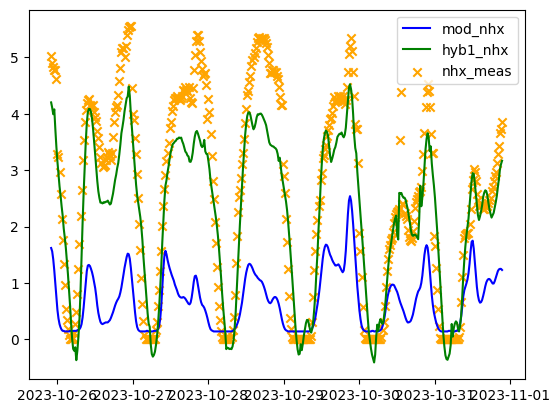
Figure 1.

# get the errors for the second round of data-driven modelling
err2 = hyb1_nhx - nhx_meas
err2 = savgol_filter(err2, 7, 3)

index = X_raw.iloc[-(len(err2)+hrt_time_steps):].index
index = index[:-hrt_time_steps]

err2 = pd.DataFrame(err2, index=index, columns=[str(test_tank[0]) + '_err2'])

To take it one step further, we look at the remaining NHx residuals again, build another data-driven model based on FFT, and correct for the errors again. We do another grid search to find the right window over which we identify the frequencies and the number of frequencies to search for. The right window width and number of frequencies is based on which combination results in the lowest custom loss. At the end, we get to see what the top frequencies look like that we leverage to make the forecast.

!pip install darts


# import required libraries/modules for FAST FOURIER TRANSFORM
from darts import TimeSeries
from darts.models.forecasting.fft import FFT
from sklearn.metrics import mean_squared_error


# find the right window size and number of frequencies for making the FFT forecast
forecast_horizon = hrt_time_steps
fft_data = TimeSeries.from_series(err2)

def eval_fft(window_size, n_freqs, X, forecast_horizon=forecast_horizon):

    error_list = []
    fcast_list = []
    model = FFT(nr_freqs_to_keep=n_freqs)

    for i in range(len(X) - window_size - forecast_horizon + 1):
        train = X[i:i+window_size]
        test = X[i+window_size:i+window_size+forecast_horizon]
        test = test.univariate_values()
        model.fit(train)
        fcasts = model.predict(forecast_horizon)
        fcast_list.append(fcasts.last_value())
        fcasts = fcasts.univariate_values()
        error = mean_squared_error(test, fcasts)
        error_list.append(error)

    print(f"error = {np.mean(error_list):.2f}")
    print("")
    return np.mean(error_list), fcast_list

param_grid = {
    'window_size': [36, 72, 108, 144],
    'n_freqs': [3, 5, 10, 20, 50]
}

best_error = np.inf
best_params = None


for window_size in param_grid['window_size']:
    for n_freqs in param_grid['n_freqs']:
        print(f"window_size = {window_size:.0f}")
        print(f"n_freqs = {n_freqs:.0f}")
        print("")
        error = eval_fft(window_size, n_freqs, fft_data)[0]
        if error < best_error:
            best_error = error
            best_params = {'window_size': window_size, 'n_freqs': n_freqs}

print("Best parameters:", best_params)


fft = eval_fft(best_params['window_size'], best_params['n_freqs'], fft_data)[1]


# find the hybrid nhx based on error forecasts and mechanistic modelled nhx
hyb2_nhx = hyb1_nhx[-len(fft):] - fft


# plot the data
x = x[-len(fft):]

plt.plot(x, mod_nhx[-len(fft):], color='blue')
plt.plot(x, hyb1_nhx[-len(fft):], color='green')
plt.scatter(x, nhx_meas[-len(fft):], color='orange', marker='x')
plt.plot(x, hyb2_nhx, color='k')
plt.legend(['mod_nhx', 'hyb1_nhx', 'nhx_meas', 'hyb2_nhx'])
plt.show()

Figure 2.

# find what the top 10 frequencies look like on the Power Spectrum
fft_result = np.fft.fft(err2)
frequencies = np.fft.fftfreq(len(err2))
frequencies = frequencies[frequencies >= 0]

sorted_freq_indices = np.argsort(frequencies)
sorted_frequencies = frequencies[sorted_freq_indices]
sorted_power_spectrum = np.abs(fft_result[sorted_freq_indices]) ** 2

normalized_power_spectrum = sorted_power_spectrum / np.sum(sorted_power_spectrum)

max_freq_indices = np.argsort(normalized_power_spectrum, axis=0)[-best_params['n_freqs']:]
max_freq_x = sorted_frequencies[max_freq_indices]
max_freq_y = normalized_power_spectrum[max_freq_indices]

plt.scatter(max_freq_x, max_freq_y, color='red', label = 'Top 10 Values')
plt.plot(sorted_frequencies, normalized_power_spectrum)
plt.xlabel('Frequency (Hz)')
plt.ylabel('Normalized Power')
plt.title('Power Spectrum')
plt.grid(True)
plt.savefig(tank + '_plot.png', dpi=300)
plt.show()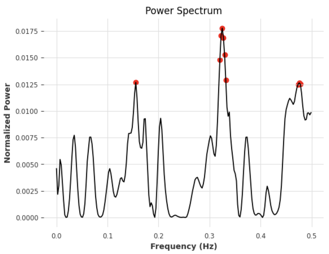

Figure 3.

Following deployment of the model for process control, the mean absolute ABAC controller error dropped from 0.81 mg/L to 0.2 mg/L

Code deep dive video. Link to access code.