Carbon Diversion: High-rate Contact Stabilization
Blue Plains Advanced Wastewater Treatment Plant (BP AWWTP) employes High-rate Contact Stabilization (HiCS) for secondary treatment following chemically enhanced primary treatment (CEPT). It precedes the tertiary treatment where nitrogen removal is performed. In addition to the primary effluent, the HiCS system receives two return flows that are hypothesized to influence performance: (i) the solids processing line (SPB) produced during the thickening and dewatering processes, and (ii) waste nitrification sludge (WNS) from the downstream tertiary nitrification process. At BP AWWTP, it was observed that bio-augmenting the A-stage HiCS process with WNS may positively influence settleability and overall process performance, whereas supernatant return flow from solids processing (SPB) may negatively influence process stability.
Unfortunately, current mechanistic modeling approaches are inadequate for robust prediction of dynamic behavior in HiCS. Therefore, the ultimate goal of this work is to develop a data-driven tool to control the secondary treatment process to keep its effluent suspended solids (ESS) below 25 mg/L.
This goal can be achieved through a two-step process:
Objective 1: Develop a data-driven model that links HiCS operational conditions and ESS. For this model to serve the goal of controlling the process ESS, the project team subjected model developement to two specific constraints:
Successfully capture ESS daily dynamics.
Identify sensitivities to changes in the manipulated variables (SPB and WNS flow rates).
Objective 2: Based on the developed model, develop a decision-making tool to inform operators with effect and optimal SPB and WNS flow rates to control ESS below 25 mg/L.

Figure 1. Modelling framework for Data-driven control of return flows of HiCS system
Get Data:
These variables were collected from multiple sources using different methods and with different collection frequencies. The DCS-based data are collected from online sensors and available with high frequency on a daily basis. This includes different flow rates like SPB flow rate (SPB_Q) and WNS flow rate (WNS_Q), dissolved oxygen (DO) concentration via online sensors, and mixed liquor suspended solids (MLSS) probe data. The second group of the data is collected and measured manually by the DC Water Lab team, but is available at a relatively high frequency (more than once a week). This includes parameters like lab-based MLSS measurements, primary effluent total suspended solids (PE_TSS), and total soluble phosphorus of the primary effluent (PE_TSP) and secondary effluent (SE_TSP). The last group of data sources requires more complex experimental measurements and is performed by the DC Water Research team, and is therefore available in a less frequent and a less systematic manner (generally available once a week.) This includes parameters like threshold of flocculation (TOF), sludge volume index (SVI), settling flux curves, and COD and nitrogen fractions for the primary effluent and secondary effluent. To complement historical data, a tailored 16-week experimental plan was designed and implemented to intentionally change the WNS and SPB control points and measure its impact. The purpose of this data collection campaign was to impose sufficient systematic variation in the WNS and SPB return flows to robustly assess their influence on ESS, thereby aiding in robust model development. This experimental campaign was completed at the end of November 2022.

Figure 2. Available data from different teams/sources
A major challenge with the data is the high degree of missingness and inconsistency in such missingness. This challenge was multiplied with data during COVID periods, where sampling frequency and routine varied significantly. Missingness was assessed using missingo library as shown below
plt.show(msno.matrix(ALL_df))
plt.show(msno.matrix(ALL_df.iloc[:,:31]))
plt.show(msno.matrix(ALL_df.iloc[:,31:62]))
plt.show(msno.matrix(ALL_df.iloc[:,62:90]))
plt.show(msno.matrix(ALL_df.iloc[:,90:]))

Figure 3. Missing instances within the dataset
(each column represents one variable, and each grey bar represents an available instance)
Prepare Data:
The main data preparation or pre-processing step was data imputation. For such a process, For data imputation, a multi-step approach was adopted. In the first step, variables were imputed using linear interpolation. This was restricted to a maximum of 2 missing consecutive days in a week (7 days). To validate the assumption that the weekly data follows a linear pattern, the data was split in weeks and a linear model was fitted into each week and the goodness of fit was evaluated to confirm its suitability. In the second step, a multivariate imputation was used to leverage the high dimensionality and co-linearity in the dataset. First, variables were selected using maximum relevance minimum redundancy (mRMR) method. Next, an optimized Huber regression model was trained using the existing points and the fitted model was used to predict the missing values. Huber regression is a robust linear regression technique used in statistics and machine learning for modeling the relationship between variables in the presence of outliers and influential data points. A threshold of prediction accuracy (validation R2 above 0.5) was set to avoid imputing variables using inaccurate models. An example of the results of the multivariate imputation is shown in Figure 5.4.4. The last step was using the moving average for variables expected to remain constant for a specific period of time. This period of time was determined according to process knowledge. For primary effluent characteristics, no imputation was performed at this step as there is no prior knowledge of changes in influent characteristics. Seven days moving average were used to impute variables related to SPB and WNS streams as they are generated based on relatively slow processes, while 3 days moving average were used for the HiCS process conditions like sludge characteristics as this was the average SRT of the system.
Given the stochastic and dynamic nature of the ESS, it was smoothed by using a 7-day rolling average. This fits well with the project objectives as the goal is to make weekly or bi-weekly decisions on SPB and WNS flow rates. The dataset was normalized using a Min-Max scaler, to ensure all values were between 0 and 1, which significantly improved model performance by ensuring that all variables contribute equally.
Train Models:
Feature selection was performed in multiple steps. The first step is selecting variables with missing ratio equal or less than 50%. Such variables were used in preliminary algorithm selection and as a starting point. Then, the artificial contrasts with ensembles (ACE) method was used for the selection of the key variables from the variables with a missing ratio below 50%. ACE is unsupervised and does not require a pre-selected number of variables or pre-determined stopping criteria. It works by first estimating feature importance using an algorithm of ensemble of trees (RF was used). Then, for each variable in the dataset, an artificial random variable (called “artificial contrast variable”) is created from the same distribution as its corresponding variable but is independent of the target. A variable is eliminated if it has lower importance, that is artificial contrast. A snippet of the code is shown below.
###########Step 1: create the HF feature with 50% missing ratio
df_HF = df_learn.copy() #Dataframe to use
threshold = 0.5 * len(df_HF)  # Set threshold
df_trgt = df_HF.dropna(axis=1, thresh=threshold) #dataframe obtained after intial filtering
df_org = df_learn.copy() #dataframe that contains Learning data with all columns

###########Step 2: Feature elimination
#Preparing the Dataframe
df_trgt_BFS = df_trgt.dropna() #drop nan
# predictor & target
X_train=df_trgt_BFS.iloc[:,:-1].sort_index()
y_train=df_trgt_BFS.iloc[:,-1].sort_index()
#scaling the Training data
X_train_sc = pd.DataFrame(MinMaxScaler().fit_transform(X_train), columns=X_train.columns)
#, index=X_train.index)
y_train_sc = pd.Series(MinMaxScaler().fit_transform(y_train.values.reshape(-1, 1)).squeeze())
#, index=y_train.index)
### Random Forest Boruta
model = RandomForestRegressor(random_state=22) ### RF used as the basis
print('boruta feature selection in progress ..........')
boruta = BorutaPy(estimator = model,
                  n_estimators = 'auto',
                  max_iter = 100, #number of trials to perform
                  verbose = 0,
                 )
boruta.fit(np.array(X_train_sc), np.array(y_train_sc))
### print results
feat_to_keep = X_train_sc.columns[boruta.support_].to_list()
feat_to_check = X_train_sc.columns[boruta.support_weak_].to_list()
### making sure SPBQ and WNSQ are included
if 'W_SPB_Q' not in feat_to_keep:
    feat_to_keep.append('W_SPB_Q')
if 'W_WNS_Q' not in feat_to_keep:
    feat_to_keep.append('W_WNS_Q')
trgt_fts = feat_to_keep + [df_org.columns[-1]] #feat_to_check given that pruning will be done
feat_to_drop = [col for col in X_train_sc.columns if col not in feat_to_keep]
# and col not in feat_to_check]
printb(f'features To be dropped based on Boruta Feature Selection:')
print(f'{feat_to_drop}')
print('============================================================================
=================================')
#Dataframe after pruning
df_trgt_B = df_org[trgt_fts]
Following this, a modified Wrapper Dominating Hybrid Sequential Forward Floating Search (incremental learning for short) method was used. In this method, variables were added to the dataset in a sequential manner. Every time a variable is added, model performance is evaluated. If improved, permutation feature importance is calculated and the variable with least importance is dropped. If performance improved, this variable is dropped, and permutation feature importance is determined again. This process is repeated until the performance is not improving. If performance did not improve by dropping variables, the added variable is selected without dropping any variables. The incremental learning process for one of the iterations is shown in Figure 5.4.7. This process continues until the samples to features ratio (S/F ratio) is less than 10. While there is no clear threshold for the S/F ratio, it is widely reported that at least S/F ratio of 10 is needed for reliable and generalizable results. Example of the code and results is shown below.
###########Step 3: Incremental Learning

#define feature space for Feedforward Feature selection
Cand_fts = [feat for feat in df_org.columns[:-1] if feat not in df_trgt.columns[:-1]]
#Dataframe to show results
FSelect_results = pd.DataFrame(index=['Feature', 'Added', 'Feature_Dropped','Data_name',
'model_name', 'Data_length','SF_ratio',
'CV_R2_val','CV_stdR2_val','CV_RMSE_val','CV_stdRMSE_val',
'CV_R2_train','CV_stdR2_train','CV_RMSE_train','CV_stdRMSE_train',
'CV_Overfit','Fit_R2','RMSE_Red','Fit_RMSE'])

for n in range(1,10000):
    df_data=pd.DataFrame(columns=['df_names','Data','Data_imb','Imbalance','Weights','log',
'meths'])
    # add starting data
    if n == 1:
        printb(f'        ============ Evaluating Control & Pruned Dataset ============')
        df_data=df_data._append({'df_names':'Ldf_Control','Data': df_trgt,'Data_imb':df_trgt,
                                 'Imbalance':False,'Weights':False,'log':False,'meths':1}
                                ,ignore_index=True)
        df_data=df_data._append({'df_names':'Ldf_Pruning','Data': df_trgt_B,'Data_imb':df_trgt_B,
                                 'Imbalance':False,'Weights':False,'log':False,'meths':1}
                                ,ignore_index=True)
        df_trgt_F = df_trgt_B.copy()
        df_new = df_trgt_B.copy()
    else:
       #Selecting the feature to add
        ft = filter_feat(Cand_fts,df_org,df_trgt_F)
        Cand_fts = [feat for feat in Cand_fts if feat != ft] #droping the feature from the list
        printb(f'        ============ Evaluating for feature {ft} ============')
        df_new = insert_S (df_org[ft],df_trgt_F,ft,post=1)
        df_data=df_data._append({'df_names':f'Ldf_{ft}','Data': df_new,'Data_imb':df_new,
                                 'Imbalance':False,'Weights':False,'log':False,'meths':1}
                                ,ignore_index=True)

        # droping features with redundancy above 0.7
        red_cols=[]
        for col in df_new.columns[:-1]:
            if col not in ['W_SPB_Q','W_WNS_Q',ft]:
                ins = ins_df(df_org,ft,col)
                p_corr=pearsonr(ins['target'],ins['feat'])[0]
                sp_corr=spearmanr(ins['target'],ins['feat'])[0]
                if abs(p_corr) > 0.7 or abs(sp_corr) > 0.7:
                    red_cols.append(col)
        print(f'red_cols : {red_cols}')
        if len(red_cols) > 0:
            df_new_red = df_new.drop(columns=red_cols)
            df_data=df_data._append({'df_names':f'Ldf_{ft}_red','Data': df_new_red,
'Data_imb':df_new_red,'Imbalance':False,'Weights':False,'log':False,'meths':1},ignore_index=True)
        else:
            printb(f'>>>>>>>>>>>>>>>>>>>>>>>>>> No Redundancy reduction for {ft} <<<<<<<<<<<
            <<<<<<<<<<<<<<<<<<')

    Comp_df=pd.DataFrame()
    m_name = 'SVM'
    for data_name,df_Lrn,df_Lrn_imb in zip(df_data['df_names'],df_data['Data'],
              df_data['Data_imb']):

        printb(f'Estimating {data_name} using SVM ..................')
        if n == 1:
            if data_name == f'Ldf_Control':
                ft = 'Cont'
            else:
                ft = 'Prn'
        Results = f'r_{ft}_{data_name}_{m_name}'
        results = f'{ft}_{data_name}_{m_name}'
        globals()[Results] = Regr_inner(df_Lrn,df_Lrn_imb,SVR,df_org=WEST_df, #inputs
                            df_name =data_name,model_name = m_name, #labels
                            scaleX=MinMaxScaler(),scaleY=MinMaxScaler(),#scaling method
                            Testing=False,Training=True,figures=False, #what to show
                            Outlier=False, #Do outlier removal or not
                            imbalance=False,weights=False,meth=1,log=False, # Do data balance treatment or not
                            r_g='G', #grid search
                            r_iter=100, # n iteration for random search
                            cv_folds=3,#Kfold_split(df_train,z_dfs,cv_folds=cv_folds), #cross validation
                            score={'R2':'r2','RMSE':'neg_root_mean_squared_error'},score2='R2',#grid search scoring
                            defaults={'kernel':'rbf'}, hyper={}, # hyperparamter and model defaults
                            threshold=0.0, #r2 threshold to consider the model in results
                            feat_imp=True,n_feat=50, #permutation feature importance
                                       )
Figure 4. Feature selection results
Following, a rigorous hyperparameter optimization (HPO) was performed along with different methods for data imbalance treatment. Below is the hyperparameter space used for optimization.
hyperp=[
        {'rmodel__C':[1,5,10],
         'rmodel__epsilon':[0.05,0.1,0.2,1,5],
         'rmodel__gamma':['auto','scale',0.001,0.1,1,5,10]}#9-SVM
        ]
An observation from data exploration is data imbalance. This is a typical challenge with data obtained from wastewater treatment. In most of the days, the process is performing well, and ESS is below 25 mg/L, as a result, the algorithm prioritizes predicting the common low values and ignores the high values. To fix this issue, several imbalance treatment methods were tested, including Synthetic Minority Oversampling Technique (SMOTE), Adaptive Synthetic Oversampling (ADASYN), weight-adjusted loss function, and quantile transformation of the target. SMOTE is an oversampling method that creates synthetic samples using k-nearest neighbors of the minority instances in the original dataset, thus addressing imbalances in the target variable distribution. ADASYN is similar to SMOTE, but instead of oversampling the minority instances of the data, it generates more samples similar to those that are difficult to learn. A weight-adjusted loss function assigns different weights to instances based on their representation in the dataset, penalizing errors associated with the less represented instances more heavily to improve model performance. This was performed by assigning weights equal to the inverse of the probability density function of the training data or by assigning higher weights to values beyond the interquartile range. Quantile transformation of the target involves transforming the target variable to follow a uniform or normal distribution, stabilizing variance and making the modeling process more robust to imbalanced data.
To train and evaluate models based on different data imbalance methods, Nested cross validation was used to compare models.
#Model Training
Reg=reg_model(**defaults)
if quantile:
   qt = QuantileTransformer(output_distribution='normal', random_state=0)
   pipe = Pipeline(steps=[("transformer", qt),("scaler", scaleX),("rmodel", Reg)])
else:
   pipe = Pipeline(steps=[("scaler", scaleX),("rmodel", Reg)])

        #inner_cross validation
        if cv_split:
            if cv_eq == 'G':
                if imbalance != False:
                    c_val = Groupshufflue_split (X_imb,g_size=g_size,
n_splits=in_cv_folds,test_size=test_size)
                else:
                    c_val = Groupshufflue_split (X_train,g_size=g_size,
n_splits=in_cv_folds,test_size=test_size)
        else:
            c_val=KFold(n_splits=in_cv_folds,shuffle=True)

        # HPO optimization:
        # Search algorithm used
        if r_g == 'R':
            grid = RandomizedSearchCV(pipe,hyper,n_iter=r_iter,cv=c_val,
                                      scoring=score,refit=score2,return_train_score=True,
                                      n_jobs=-1)
        if r_g == 'G':
            grid = GridSearchCV(pipe,hyper,cv=c_val,scoring=score,refit=score2,
                  return_train_score=True,n_jobs=-1)
Modeling Results:
In the actual project, 10 different algorithms were tested. However, in the modelling notebook only support vector machines are used as an example. The best results were obtained with weight adjusted loss function. This applies to both goodness of fit indicated by R2 and RMSE, and degree of overfitting measured as the percentage of the decrease in R2 from training to testing.
Table 1. SVM model results at different imbalance treatment methods

Below are the plots for such model “SVM_W3”.


Figure 5. Final model results
(top: predicted vs actual results, bottom: time series results)
For this model, permutation feature importance was determined to understand which variables are more valuable to the model. This is particularly significant because the ultimate goal is to use this model to advise on SPB and WNS flow rates. Below is snippet of the code and the results
def feature_importance_permutation (model, y_test, X_test,n_iteration=100,
figures=False,log=False):
    original_rmse = np.sqrt(mean_squared_error(y_test, model.predict(X_test)))

    # Calculate permutation feature importance
    permuted_rmses = []
    permuted_rmse_stds = []  # To store standard deviations

    for feature_name in X_test.columns:
        feature_permuted_rmses = []
        for _ in range(n_iteration):
            # Make a copy of the original feature
            permuted_X_test = X_test.copy()
            # Shuffle the values of the current feature
            permuted_X_test[feature_name] = np.random.permutation(permuted_X_test[feature_name])
            # Calculate predictions on the permuted data
            permuted_predictions = model.predict(permuted_X_test)
            #permuted_predictions = scaler_Y.inverse_transform(p_p.reshape(-1,1)).squeeze()
            if log:
                permuted_predictions=np.exp(permuted_predictions)
            permuted_rmse = np.sqrt(mean_squared_error(y_test, permuted_predictions))
            feature_permuted_rmses.append(permuted_rmse)

        # Calculate the average and standard deviation of RMSE over iterations for the current feature
        avg_permuted_rmse = np.mean(feature_permuted_rmses)
        std_permuted_rmse = np.std(feature_permuted_rmses)
        permuted_rmses.append(avg_permuted_rmse)
        permuted_rmse_stds.append(std_permuted_rmse)

    # Calculate feature importance scores
    feature_importances = ((original_rmse - np.array(permuted_rmses)) / original_rmse) * -100
    # Create a DataFrame to store the feature importance scores and standard deviations
    feature_importance_df = pd.DataFrame({
        'Feature': X_test.columns,
        'Average Permuted RMSE': permuted_rmses,
        'Std Deviation RMSE': permuted_rmse_stds,
        'Importance': feature_importances
    })

    # Rank the features based on importance
    ranked_feature_importance_df = feature_importance_df.sort_values(by='Importance',
    ascending=False)
    ranked_feature_importance_df.set_index('Feature', drop=False, inplace=True)

    #display(ranked_feature_importance_df)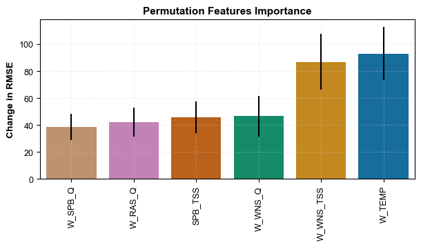
Figure 6. Results of feature importance of the final model
Project overview video
Define Problem:
Deploy Model:
As mentioned earlier, our ultimate objective is to use the developed model as an offline decision-making tool to inform operators about how to manage WNS and SPB flowrates to reduce ESS or at least keep it below 25 mg/L. However, it can be implied from the feature importance result that ESS is affected more by the temperatures and WNS total suspended solids (WNS TSS) than SPB and WNS flow rates.
Therefore, the developed tool shall answer two questions for the operators. The first question is “under the existing conditions, are the existing WNS and SPB flowrates contributing to the observed ESS”, while the second question is “under the existing conditions, how will ESS change if WNS and SPB flowrates change”.
The suggested deployment tool will rely on the pre-trained model. This model can be re-trained on a monthly or bi-weekly basis according to the data collection. To answer the first question, Shaply can be used to identify the current contribution of each variable, as shown in the figures below.

Figure 7. Instance-based SHAP results for two different days
In addition, the model can be fed the current conditions (the input variables) as a new instance in addition to all possible flow rates for WNS and SPB, and the algorithm will generate different predictions according the WNS and SPB values. These values can be plotted in a heat map similar to the one shown below. The center of the heatmap can be adjusted based on the current ESS. This heat map will answer both questions; if all values are similar to the existing ESS, this means WNS and SPB return flows are not the main contributors to ESS. For the second question, the heat map will identify the zones of operation where low ESS is expected under the existing conditions.

Figure 8. Heatmap of the results of the final model under typical operational conditions
Code overview video. Link to access code.